Getting Started#
We’re going to use a standard hierarchical Bayesian model and the rectified-logistic function to estimate neural recruitment curves.
A Simple Example#
Tip
If you have trouble running the commands in this tutorial, please copy the command and its output, then open an issue on our GitHub repository. We’ll do our best to help you!
Begin by reading the mock_data.csv file:
import pandas as pd

url = "https://raw.githubusercontent.com/hbmep/hbmep/refs/heads/docs-data/data/mock_data.csv"
df = pd.read_csv(url)
df shape:		(245, 4)
df columns:		TMSIntensity, participant, PKPK_ECR, PKPK_FCR
All participants:	P1, P2, P3

First 5 rows:

   TMSIntensity participant  PKPK_ECR  PKPK_FCR
0         43.79          P1     0.197     0.048
1         55.00          P1     0.224     0.068
2         41.00          P1     0.112     0.110
3         43.00          P1     0.149     0.058
4         14.00          P1     0.014     0.011
This dataset contains TMS responses (peak-to-peak amplitude, in mV) for three participants (P1, P2, P3), recorded from two muscles (ECR and FCR).
The column TMSIntensity represents stimulation intensity in percent maximum stimulator output (0–100% MSO).
Build the model#
Next, we initialize a standard hierarchical Bayesian model. This step typically consists of assigning the model’s attributes to the appropriate dataframe columns, setting the sampling parameters, and choosing the recruitment curve function.
import hbmep as mep

model = mep.StandardHB()

# Point to the respective columns in dataframe
model.intensity = "TMSIntensity"
model.features = ["participant"]
model.response = ["PKPK_ECR", "PKPK_FCR"]

# Specify the sampling parameters
model.mcmc_params = {
    "num_chains": 4,
    "thinning": 1,
    "num_warmup": 1000,
    "num_samples": 1000,
}

# Set the function
model._model = model.rectified_logistic
Running the model#
Before fitting the model, we can visualize the dataset. Since the plot is saved as a PDF, we need to specify an output path.
import os

# Create the output directory
current_dir = os.getcwd()
output_dir = os.path.join(current_dir, "hbmep-getting-started")
os.makedirs(output_dir, exist_ok=True)

# Plot dataset and save it as a PDF
output_path = os.path.join(output_dir, "dataset.pdf")
model.plot(df, output_path=output_path)
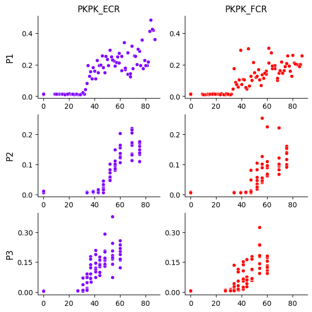
The plot shows rows as participants and columns as muscles. The x-axis is TMS intensity (% MSO), and the y-axis is MEP peak-to-peak amplitude (mV).
Next, we process the dataframe by encoding categorical feature columns. This returns the same dataframe with encoded values, plus an encoder dictionary for mapping back to original labels.
# Process the dataframe
df, encoder = model.load(df)
Encoded participants:	0, 1, 2
Participant mapping:	0 -> P1, 1 -> P2, 2 -> P3
Now we run the model to estimate curves.
# Run
mcmc, posterior = model.run(df=df)

# Check convergence diagnostics
summary_df = model.summary(posterior)
print(summary_df.to_string())
Show code cell output
2026-04-19 01:43:21,770 - hbmep.util.util - INFO - func:trace took: 1.05 sec
2026-04-19 01:43:21,770 - hbmep.model.base_model - INFO - Running...
Compiling.. :   0%|          | 0/2000 [00:00<?, ?it/s]


Running chain 0:   0%|          | 0/2000 [00:01<?, ?it/s]


Running chain 0:   5%|▌         | 100/2000 [00:04<00:57, 33.25it/s]


Running chain 0:  10%|█         | 200/2000 [00:05<00:30, 58.37it/s]


Running chain 0:  15%|█▌        | 300/2000 [00:06<00:20, 84.27it/s]


Running chain 0:  20%|██        | 400/2000 [00:06<00:14, 107.57it/s]


Running chain 0:  25%|██▌       | 500/2000 [00:07<00:11, 127.38it/s]


Running chain 0:  30%|███       | 600/2000 [00:07<00:09, 153.86it/s]


Running chain 0:  35%|███▌      | 700/2000 [00:08<00:07, 182.40it/s]


Running chain 0:  40%|████      | 800/2000 [00:08<00:05, 205.34it/s]


Running chain 0:  45%|████▌     | 900/2000 [00:08<00:05, 219.28it/s]
Running chain 0:  50%|█████     | 1000/2000 [00:09<00:04, 221.30it/s]


Running chain 0:  55%|█████▌    | 1100/2000 [00:09<00:04, 213.59it/s]


Running chain 0:  60%|██████    | 1200/2000 [00:10<00:03, 212.54it/s]


Running chain 0:  65%|██████▌   | 1300/2000 [00:10<00:03, 211.98it/s]


Running chain 0:  70%|███████   | 1400/2000 [00:11<00:02, 201.64it/s]


Running chain 0:  75%|███████▌  | 1500/2000 [00:11<00:02, 201.41it/s]


Running chain 0:  80%|████████  | 1600/2000 [00:12<00:01, 201.20it/s]


Running chain 0:  85%|████████▌ | 1700/2000 [00:12<00:01, 201.82it/s]


Running chain 0:  90%|█████████ | 1800/2000 [00:13<00:01, 196.21it/s]


Running chain 0:  95%|█████████▌| 1900/2000 [00:13<00:00, 193.55it/s]


Running chain 0: 100%|██████████| 2000/2000 [00:14<00:00, 139.46it/s]


Running chain 3: 100%|██████████| 2000/2000 [00:14<00:00, 138.52it/s]

Running chain 2: 100%|██████████| 2000/2000 [00:14<00:00, 134.86it/s]
Running chain 1: 100%|██████████| 2000/2000 [00:15<00:00, 129.55it/s]
2026-04-19 01:43:37,559 - hbmep.util.util - INFO - func:run took: 16.84 sec
2026-04-19 01:43:37,684 - hbmep.util.util - INFO - func:summary took: 0.12 sec
                mean     sd  hdi_2.5%  hdi_97.5%  mcse_mean  mcse_sd  ess_bulk  ess_tail  r_hat
a_loc         35.418  5.576    24.891     47.705      0.157    0.299    2321.0     869.0    1.0
a_scale       11.170  7.101     3.772     25.594      0.231    0.376    1611.0    1203.0    1.0
b_scale        0.189  0.115     0.061      0.381      0.003    0.013    1563.0    1594.0    1.0
g_scale        0.013  0.005     0.006      0.024      0.000    0.000    1047.0     975.0    1.0
h_scale        0.282  0.129     0.120      0.524      0.004    0.007    1054.0    1250.0    1.0
v_scale        4.547  2.913     0.246     10.230      0.050    0.040    2554.0    1966.0    1.0
c₁_scale       3.008  2.633     0.075      8.490      0.051    0.045    2077.0    2303.0    1.0
c₂_scale       0.280  0.102     0.125      0.493      0.003    0.003    1194.0    1728.0    1.0
a[0, 0]       31.900  0.463    30.731     32.637      0.016    0.021    1815.0     754.0    1.0
a[0, 1]       31.609  0.538    30.537     32.577      0.011    0.010    2845.0    2277.0    1.0
a[1, 0]       45.521  0.870    43.650     46.427      0.034    0.069    1385.0     650.0    1.0
a[1, 1]       44.842  0.815    43.216     46.156      0.017    0.022    2870.0    2747.0    1.0
a[2, 0]       30.066  0.431    29.251     30.719      0.010    0.022    2563.0    1600.0    1.0
a[2, 1]       31.175  0.673    29.987     32.482      0.012    0.020    3614.0    2677.0    1.0
b_raw[0, 0]    1.118  0.479     0.330      2.112      0.011    0.007    1767.0    1753.0    1.0
b_raw[0, 1]    1.372  0.550     0.419      2.458      0.010    0.009    2899.0    2533.0    1.0
b_raw[1, 0]    0.607  0.356     0.078      1.335      0.010    0.009    1399.0    2050.0    1.0
b_raw[1, 1]    0.495  0.312     0.040      1.110      0.006    0.006    1912.0    2230.0    1.0
b_raw[2, 0]    0.570  0.305     0.101      1.193      0.007    0.007    1773.0    2025.0    1.0
b_raw[2, 1]    0.321  0.215     0.024      0.743      0.005    0.005    1879.0    2145.0    1.0
g_raw[0, 0]    1.187  0.389     0.453      1.915      0.012    0.007    1048.0     983.0    1.0
g_raw[0, 1]    1.127  0.372     0.457      1.859      0.011    0.007    1038.0    1049.0    1.0
g_raw[1, 0]    0.746  0.246     0.303      1.226      0.007    0.005    1056.0     957.0    1.0
g_raw[1, 1]    0.640  0.215     0.254      1.063      0.006    0.004    1092.0    1102.0    1.0
g_raw[2, 0]    0.569  0.202     0.202      0.955      0.006    0.003    1123.0    1105.0    1.0
g_raw[2, 1]    0.692  0.243     0.274      1.198      0.007    0.004    1128.0    1148.0    1.0
h_raw[0, 0]    0.981  0.359     0.372      1.716      0.011    0.006    1053.0    1225.0    1.0
h_raw[0, 1]    0.665  0.244     0.244      1.165      0.007    0.004    1056.0    1246.0    1.0
h_raw[1, 0]    0.769  0.304     0.251      1.373      0.009    0.006    1076.0    1308.0    1.0
h_raw[1, 1]    0.649  0.313     0.170      1.260      0.007    0.008    1423.0    1490.0    1.0
h_raw[2, 0]    0.941  0.369     0.295      1.657      0.010    0.006    1191.0    1458.0    1.0
h_raw[2, 1]    0.991  0.464     0.234      1.933      0.010    0.008    1952.0    2093.0    1.0
v_raw[0, 0]    0.975  0.597     0.077      2.158      0.008    0.010    3906.0    2311.0    1.0
v_raw[0, 1]    0.936  0.606     0.039      2.113      0.008    0.009    3781.0    2116.0    1.0
v_raw[1, 0]    0.646  0.598     0.000      1.819      0.014    0.009    1059.0     727.0    1.0
v_raw[1, 1]    0.755  0.603     0.001      1.946      0.010    0.009    2017.0    1373.0    1.0
v_raw[2, 0]    0.786  0.608     0.001      1.977      0.010    0.009    2269.0    1195.0    1.0
v_raw[2, 1]    0.780  0.602     0.001      1.962      0.009    0.009    2906.0    2006.0    1.0
c₁_raw[0, 0]   0.932  0.592     0.045      2.082      0.009    0.009    3525.0    2086.0    1.0
c₁_raw[0, 1]   0.927  0.598     0.031      2.074      0.008    0.009    3902.0    2410.0    1.0
c₁_raw[1, 0]   0.704  0.621     0.002      1.893      0.011    0.010    1953.0    1767.0    1.0
c₁_raw[1, 1]   0.822  0.581     0.006      1.919      0.009    0.009    3242.0    2062.0    1.0
c₁_raw[2, 0]   0.318  0.490     0.002      1.418      0.011    0.011    1553.0    3387.0    1.0
c₁_raw[2, 1]   0.799  0.600     0.009      2.003      0.008    0.009    3473.0    2772.0    1.0
c₂_raw[0, 0]   0.300  0.112     0.116      0.526      0.003    0.002    1364.0    1744.0    1.0
c₂_raw[0, 1]   0.503  0.187     0.186      0.869      0.005    0.004    1330.0    1477.0    1.0
c₂_raw[1, 0]   0.335  0.131     0.115      0.577      0.004    0.003    1304.0    2088.0    1.0
c₂_raw[1, 1]   0.917  0.332     0.341      1.555      0.009    0.006    1383.0    1902.0    1.0
c₂_raw[2, 0]   1.239  0.464     0.462      2.167      0.010    0.007    1947.0    2264.0    1.0
c₂_raw[2, 1]   1.351  0.469     0.523      2.266      0.012    0.008    1368.0    1682.0    1.0
Generate posterior predictive#
Before plotting the curves, we have to generate predictions using the posterior. The following returns the posterior predictive distribution.
# Create prediction dataframe
prediction_df = model.make_prediction_dataset(df=df, num_points=1000)

# Use the model to predict on the prediction dataframe
predictive = model.predict(df=prediction_df, posterior=posterior)
Visualizing the curves#
We can use the posterior predictive to plot the estimated curves. Again, we specify the path where the generated PDF will be stored.
# Plot estimated curves
output_path = os.path.join(output_dir, "curves.pdf")
model.plot_curves(
    df=df,
    prediction_df=prediction_df,
    predictive=predictive,
    posterior=posterior,
    encoder=encoder,
    output_path=output_path
)
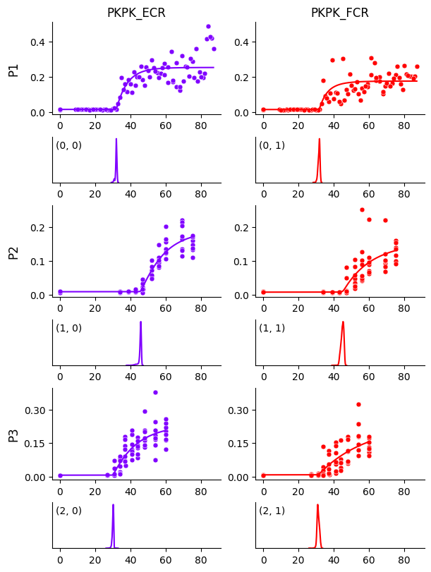
In each panel above, the top plot shows the estimated curve overlaid on data, and the bottom plot shows the posterior distribution of the threshold parameter.
We can also plot 95% highest density intervals (HDIs) around the curves to see if they contain most of the data. This is done by passing predictive_hdi_prob=0.95 to the plot_curves method.
# Plot observations HDI
output_path = os.path.join(output_dir, "obs_hdi.pdf")
model.plot_curves(
    df=df,
    prediction_df=prediction_df,
    predictive=predictive,
    posterior=posterior,
    encoder=encoder,
    output_path=output_path,
    predictive_hdi_prob=0.95
)
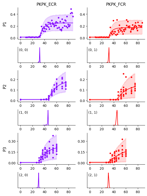
Mixture extension#
The curves look good overall, except for participant P1 and muscle FCR, where the growth rate seems to be biased by a few data points. This can be addressed with a mixture model. To enable it, we can add the following line at the end of the model-building code:
# Enable mixture model
model.use_mixture = True
For a complete example, see Mixture Extension.
Accessing parameters#
Each participant, muscle combination is assigned a tuple index, which can be used to access the curve parameters, which are stored in the posterior dictionary as NumPy arrays.
Here we show how to access the threshold parameter.
# Threshold parameter
a = posterior[mep.site.a]
Shape of a:	(4000, 3, 2)

First dimension corresponds to the number of samples:		4000
Second dimension corresponds to the number of participants:	3
Last dimension corresponds to the number of muscles:		2
By default, we have 4000 posterior samples (4 chains, 1000 samples each). We can set more chains or samples by updating the model-building code:
# Use 4 chains, 2000 samples each, for a total of 8000 samples
model.mcmc_params = {
    "num_chains": 4,
    "thinning": 1,
    "num_warmup": 2000,
    "num_samples": 2000,
}
The other curve parameters can be accessed similarly using their keys.
print(f"{mep.site.b} controls the growth rate")
print(f"{mep.site.g} is the offset")
print(f"({mep.site.g} + {mep.site.h}) is the saturation")
b controls the growth rate
g is the offset
(g + h) is the saturation
Saving the model#
We can save the model, posterior samples, and other objects using pickle for later analysis. Note that we don’t have to save the predictions as they can be generated after loading the saved model.
# Model state
model_state = model.state_dict()

# Save to output directory
mep.save(
    model_state=model_state,
    df=df,
    posterior=posterior,
    encoder=encoder,
    mcmc=mcmc,
    output_dir=output_dir
)
Loading the saved model#
A saved model can be loaded by specifying the directory where it’s saved as follows.
# Load saved objects
model_state, df, posterior, encoder, mcmc = mep.load(
    model_dir=output_dir
)

# Load model state
model = mep.StandardHB()
model.load_state_dict(model_state)
Using other functions#
Alternatively, we can use other functions to estimate the recruitment curves. The following choices are available:
logistic-4, also known as the Boltzmann sigmoid, is the most common function used to estimate recruitment curves
logistic-5 is a more generalized version of logistic-4
rectified-linear
If estimating threshold is not important, we recommend using logistic-5 over logistic-4, which has a much better predictive performance.
For example, to use logistic-5 function, we need to update the model-building code and point to it, and rest of the tutorial remains the same.
# Set the function to logistic-5
model._model = model.logistic5
For a complete example, see Using Logistic-5.