Mixture Extension#
We use the same dataset from Getting Started with a mixture model.
import os

import pandas as pd
import hbmep as mep

url = "https://raw.githubusercontent.com/hbmep/hbmep/refs/heads/docs-data/data/mock_data.csv"
df = pd.read_csv(url)
Build the model#
model = mep.StandardHB()

# Point to the respective columns in dataframe
model.intensity = "TMSIntensity"
model.features = ["participant"]
model.response = ["PKPK_ECR", "PKPK_FCR"]

# Set the function
model._model = model.rectified_logistic

# Enable mixture
model.use_mixture = True
Running the model#
# Process the dataframe
df, encoder = model.load(df)

# Run
mcmc, posterior = model.run(df=df)

# Check convergence diagnostics
summary_df = model.summary(posterior)
print(summary_df.to_string())
Show code cell output
2026-04-19 01:42:22,859 - hbmep.util.util - INFO - func:load took: 0.00 sec
2026-04-19 01:42:24,347 - hbmep.util.util - INFO - func:trace took: 1.49 sec
2026-04-19 01:42:24,348 - hbmep.model.base_model - INFO - Running...
Compiling.. :   0%|          | 0/3000 [00:00<?, ?it/s]


Running chain 0:   0%|          | 0/3000 [00:02<?, ?it/s]


Running chain 0:   5%|▌         | 150/3000 [00:06<01:26, 33.12it/s]


Running chain 0:  10%|█         | 300/3000 [00:07<00:45, 59.55it/s]


Running chain 0:  15%|█▌        | 450/3000 [00:08<00:29, 86.69it/s]


Running chain 0:  20%|██        | 600/3000 [00:09<00:22, 106.45it/s]


Running chain 0:  25%|██▌       | 750/3000 [00:10<00:17, 126.00it/s]


Running chain 0:  30%|███       | 900/3000 [00:11<00:15, 137.69it/s]


Running chain 0:  35%|███▌      | 1050/3000 [00:12<00:13, 140.77it/s]


Running chain 0:  40%|████      | 1200/3000 [00:13<00:11, 156.83it/s]


Running chain 0:  45%|████▌     | 1350/3000 [00:13<00:09, 166.06it/s]


Running chain 0:  50%|█████     | 1500/3000 [00:14<00:08, 179.40it/s]


Running chain 0:  55%|█████▌    | 1650/3000 [00:15<00:07, 192.78it/s]


Running chain 0:  60%|██████    | 1800/3000 [00:15<00:06, 196.39it/s]
Running chain 0:  65%|██████▌   | 1950/3000 [00:16<00:05, 198.03it/s]


Running chain 0:  70%|███████   | 2100/3000 [00:17<00:05, 179.16it/s]


Running chain 0:  75%|███████▌  | 2250/3000 [00:18<00:04, 172.73it/s]


Running chain 0:  80%|████████  | 2400/3000 [00:19<00:03, 166.17it/s]


Running chain 0:  85%|████████▌ | 2550/3000 [00:20<00:02, 160.66it/s]


Running chain 0:  90%|█████████ | 2700/3000 [00:21<00:01, 160.84it/s]


Running chain 0:  95%|█████████▌| 2850/3000 [00:22<00:00, 161.45it/s]
Running chain 2: 100%|██████████| 3000/3000 [00:23<00:00, 129.53it/s]


Running chain 1: 100%|██████████| 3000/3000 [00:23<00:00, 128.80it/s]
Running chain 0: 100%|██████████| 3000/3000 [00:23<00:00, 128.44it/s]


Running chain 3: 100%|██████████| 3000/3000 [00:24<00:00, 124.44it/s]
2026-04-19 01:42:48,815 - hbmep.util.util - INFO - func:run took: 25.96 sec
2026-04-19 01:42:48,946 - hbmep.util.util - INFO - func:summary took: 0.13 sec
                mean     sd  hdi_2.5%  hdi_97.5%  mcse_mean  mcse_sd  ess_bulk  ess_tail  r_hat
a_loc         36.150  6.068    25.128     48.455      0.194    0.451    2277.0     886.0   1.00
a_scale       11.756  7.281     4.030     24.846      0.251    0.513    1463.0     985.0   1.00
b_scale        0.153  0.078     0.056      0.294      0.002    0.007    1143.0    1598.0   1.00
g_scale        0.013  0.005     0.006      0.023      0.000    0.000    1181.0     859.0   1.00
h_scale        0.262  0.115     0.115      0.470      0.004    0.009    1008.0    1011.0   1.00
v_scale        5.042  3.110     0.442     11.166      0.053    0.050    2678.0    2471.0   1.00
c₁_scale       4.655  3.019     0.234     10.467      0.045    0.047    3548.0    2424.0   1.00
c₂_scale       0.169  0.062     0.078      0.292      0.002    0.002    1326.0    1684.0   1.00
a[0, 0]       31.858  0.471    30.688     32.625      0.017    0.020    1723.0     996.0   1.00
a[0, 1]       31.061  0.504    30.042     32.028      0.008    0.009    4120.0    2551.0   1.00
a[1, 0]       45.421  0.981    43.263     46.484      0.053    0.130     650.0     386.0   1.00
a[1, 1]       47.813  0.955    46.476     49.770      0.022    0.013    2335.0    3086.0   1.00
a[2, 0]       31.598  0.535    30.769     32.587      0.011    0.006    2624.0    3408.0   1.00
a[2, 1]       32.339  0.820    30.791     33.541      0.025    0.083    2490.0    2105.0   1.00
b_raw[0, 0]    1.202  0.485     0.336      2.124      0.012    0.008    1455.0    1850.0   1.00
b_raw[0, 1]    0.517  0.249     0.130      1.022      0.006    0.005    1325.0    1758.0   1.00
b_raw[1, 0]    0.726  0.396     0.141      1.540      0.015    0.014     728.0    1103.0   1.00
b_raw[1, 1]    0.740  0.385     0.098      1.473      0.009    0.007    1550.0    1881.0   1.00
b_raw[2, 0]    1.065  0.439     0.336      1.971      0.011    0.008    1371.0    1661.0   1.00
b_raw[2, 1]    0.432  0.261     0.046      0.938      0.006    0.006    1596.0    2317.0   1.00
g_raw[0, 0]    1.200  0.367     0.548      1.939      0.010    0.007    1192.0     839.0   1.00
g_raw[0, 1]    1.143  0.349     0.483      1.812      0.010    0.007    1189.0     841.0   1.00
g_raw[1, 0]    0.754  0.231     0.332      1.214      0.006    0.005    1178.0     846.0   1.00
g_raw[1, 1]    0.657  0.202     0.268      1.036      0.006    0.004    1170.0     935.0   1.00
g_raw[2, 0]    0.582  0.183     0.243      0.945      0.005    0.004    1234.0     881.0   1.00
g_raw[2, 1]    0.715  0.229     0.316      1.190      0.006    0.004    1209.0     911.0   1.00
h_raw[0, 0]    1.048  0.350     0.390      1.727      0.011    0.006    1016.0     931.0   1.01
h_raw[0, 1]    0.834  0.285     0.319      1.418      0.009    0.005    1034.0    1021.0   1.00
h_raw[1, 0]    0.800  0.287     0.291      1.378      0.009    0.006     993.0    1021.0   1.01
h_raw[1, 1]    0.584  0.216     0.188      0.993      0.006    0.005    1093.0    1005.0   1.00
h_raw[2, 0]    0.834  0.286     0.333      1.411      0.009    0.005    1053.0    1129.0   1.00
h_raw[2, 1]    0.959  0.402     0.291      1.765      0.009    0.007    1616.0    1352.0   1.00
v_raw[0, 0]    0.966  0.605     0.059      2.132      0.010    0.010    2774.0    1720.0   1.00
v_raw[0, 1]    0.927  0.591     0.042      2.028      0.008    0.010    3639.0    2305.0   1.00
v_raw[1, 0]    0.642  0.596     0.000      1.787      0.015    0.009     638.0     513.0   1.00
v_raw[1, 1]    0.831  0.592     0.009      2.000      0.009    0.010    2853.0    1652.0   1.00
v_raw[2, 0]    0.862  0.584     0.013      1.976      0.009    0.009    2890.0    1813.0   1.00
v_raw[2, 1]    0.749  0.602     0.001      1.912      0.010    0.010    1885.0    1299.0   1.00
c₁_raw[0, 0]   0.874  0.589     0.021      2.004      0.008    0.009    3370.0    1762.0   1.00
c₁_raw[0, 1]   0.828  0.588     0.014      1.972      0.009    0.009    3159.0    2005.0   1.00
c₁_raw[1, 0]   0.773  0.607     0.001      1.956      0.009    0.010    2484.0    1406.0   1.00
c₁_raw[1, 1]   0.839  0.595     0.007      1.983      0.009    0.009    3337.0    1781.0   1.00
c₁_raw[2, 0]   0.793  0.587     0.006      1.904      0.009    0.009    3171.0    1890.0   1.00
c₁_raw[2, 1]   0.845  0.603     0.013      2.007      0.009    0.009    3311.0    2107.0   1.00
c₂_raw[0, 0]   0.469  0.172     0.175      0.821      0.005    0.003    1317.0    1624.0   1.00
c₂_raw[0, 1]   0.491  0.180     0.172      0.834      0.004    0.003    1502.0    2252.0   1.00
c₂_raw[1, 0]   0.462  0.178     0.165      0.821      0.004    0.003    1457.0    2020.0   1.00
c₂_raw[1, 1]   0.614  0.238     0.216      1.097      0.006    0.004    1636.0    2131.0   1.00
c₂_raw[2, 0]   0.895  0.316     0.342      1.534      0.008    0.005    1478.0    2160.0   1.00
c₂_raw[2, 1]   1.699  0.530     0.682      2.725      0.014    0.008    1372.0    1848.0   1.00
p_outlier      0.009  0.001     0.007      0.010      0.000    0.000    3303.0    1848.0   1.00
Visualizing the curves#
# Create prediction dataframe
prediction_df = model.make_prediction_dataset(df=df, num_points=1000)

# Use the model to predict on the prediction dataframe
predictive = model.predict(df=prediction_df, posterior=posterior)

# Create the output directory
current_dir = os.getcwd()
output_dir = os.path.join(current_dir, "hbmep-mixture-extension")
os.makedirs(output_dir, exist_ok=True)

# Plot estimated curves
output_path = os.path.join(output_dir, "curves.pdf")
model.plot_curves(
    df=df,
    prediction_df=prediction_df,
    predictive=predictive,
    posterior=posterior,
    encoder=encoder,
    output_path=output_path
)

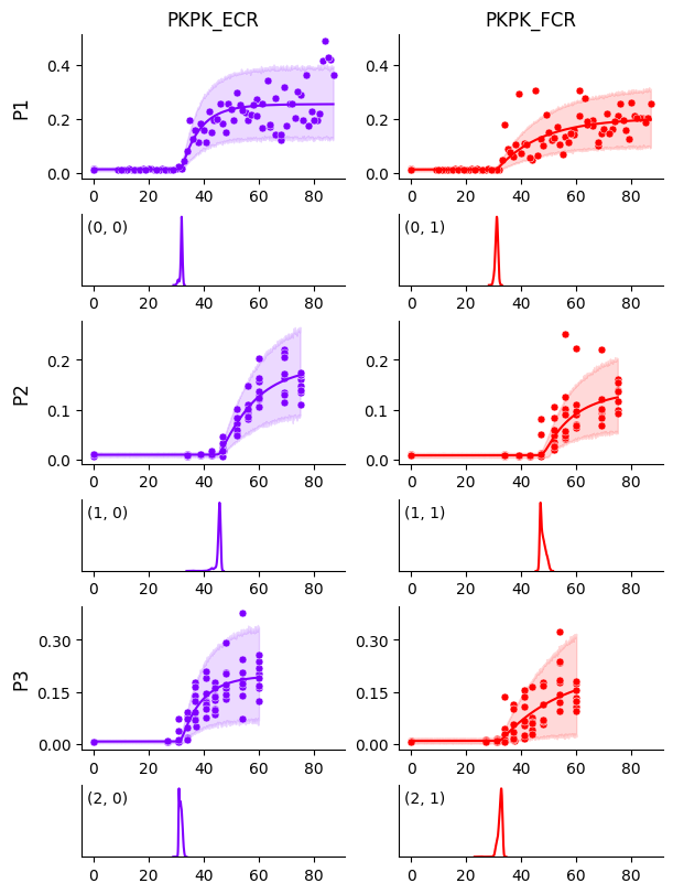
We see that the curve for participant P1 and muscle FCR is no longer biased by those few data points, compared to Getting Started. This becomes even clearer when we plot the HDIs around the curves below.
# Plot observations HDI
output_path = os.path.join(output_dir, "obs_hdi.pdf")
model.plot_curves(
    df=df,
    prediction_df=prediction_df,
    predictive=predictive,
    posterior=posterior,
    encoder=encoder,
    output_path="mixture_obs_hdi.pdf",
    predictive_hdi_var=mep.site.obs,
    predictive_hdi_prob=0.95
)