Using Logistic-5#
We use the same dataset from Getting Started with a five-parameter logistic-5 function.
import os

import pandas as pd
import hbmep as mep

url = "https://raw.githubusercontent.com/hbmep/hbmep/refs/heads/docs-data/data/mock_data.csv"
df = pd.read_csv(url)
Build the model#
model = mep.StandardHB()

# Point to the respective columns in dataframe
model.intensity = "TMSIntensity"
model.features = ["participant"]
model.response = ["PKPK_ECR", "PKPK_FCR"]

# Set the function
model._model = model.logistic5
Running the model#
# Process the dataframe
df, encoder = model.load(df)

# Run
mcmc, posterior = model.run(df=df)

# Check convergence diagnostics
summary_df = model.summary(posterior)
print(summary_df.to_string())
Show code cell output
2026-04-19 01:41:27,850 - hbmep.util.util - INFO - func:load took: 0.00 sec
2026-04-19 01:41:28,918 - hbmep.util.util - INFO - func:trace took: 1.07 sec
2026-04-19 01:41:28,918 - hbmep.model.base_model - INFO - Running...
Compiling.. :   0%|          | 0/3000 [00:00<?, ?it/s]


Running chain 0:   0%|          | 0/3000 [00:01<?, ?it/s]


Running chain 0:   5%|▌         | 150/3000 [00:04<00:53, 53.65it/s]


Running chain 0:  10%|█         | 300/3000 [00:05<00:32, 82.74it/s]


Running chain 0:  15%|█▌        | 450/3000 [00:06<00:22, 111.34it/s]


Running chain 0:  20%|██        | 600/3000 [00:07<00:19, 126.24it/s]
Running chain 0:  25%|██▌       | 750/3000 [00:08<00:15, 146.77it/s]


Running chain 0:  30%|███       | 900/3000 [00:09<00:13, 159.46it/s]


Running chain 0:  35%|███▌      | 1050/3000 [00:10<00:12, 161.49it/s]


Running chain 0:  40%|████      | 1200/3000 [00:10<00:10, 171.06it/s]


Running chain 0:  45%|████▌     | 1350/3000 [00:11<00:08, 185.99it/s]

Running chain 0:  50%|█████     | 1500/3000 [00:12<00:07, 197.91it/s]


Running chain 0:  55%|█████▌    | 1650/3000 [00:12<00:06, 198.44it/s]

Running chain 0:  60%|██████    | 1800/3000 [00:13<00:05, 212.29it/s]
Running chain 0:  65%|██████▌   | 1950/3000 [00:14<00:04, 219.40it/s]


Running chain 0:  70%|███████   | 2100/3000 [00:15<00:04, 190.71it/s]


Running chain 0:  75%|███████▌  | 2250/3000 [00:16<00:04, 174.14it/s]


Running chain 0:  80%|████████  | 2400/3000 [00:17<00:03, 166.47it/s]


Running chain 0:  85%|████████▌ | 2550/3000 [00:18<00:02, 162.86it/s]


Running chain 0:  90%|█████████ | 2700/3000 [00:19<00:01, 160.57it/s]


Running chain 0:  95%|█████████▌| 2850/3000 [00:20<00:00, 157.21it/s]


Running chain 0: 100%|██████████| 3000/3000 [00:21<00:00, 142.63it/s]

Running chain 2: 100%|██████████| 3000/3000 [00:21<00:00, 139.73it/s]
Running chain 1: 100%|██████████| 3000/3000 [00:21<00:00, 139.54it/s]


Running chain 3: 100%|██████████| 3000/3000 [00:21<00:00, 139.29it/s]
2026-04-19 01:41:50,732 - hbmep.util.util - INFO - func:run took: 22.88 sec
2026-04-19 01:41:50,857 - hbmep.util.util - INFO - func:summary took: 0.12 sec
                mean     sd  hdi_2.5%  hdi_97.5%  mcse_mean  mcse_sd  ess_bulk  ess_tail  r_hat
a_loc         42.051  6.281    29.646     55.300      0.138    0.269    2864.0    1277.0    1.0
a_scale       13.068  7.704     4.772     28.420      0.211    0.428    2332.0    1758.0    1.0
b_scale        0.597  0.347     0.173      1.249      0.011    0.017    1228.0    1332.0    1.0
g_scale        0.012  0.005     0.006      0.023      0.000    0.000     948.0     776.0    1.0
h_scale        0.225  0.099     0.098      0.407      0.004    0.007     975.0    1047.0    1.0
v_scale        0.174  0.188     0.000      0.525      0.003    0.008    3709.0    2134.0    1.0
c₁_scale       2.922  2.658     0.047      8.296      0.048    0.047    2497.0    2860.0    1.0
c₂_scale       0.284  0.106     0.131      0.504      0.003    0.003    1187.0    1685.0    1.0
a[0, 0]       35.709  0.736    34.354     37.190      0.011    0.012    4527.0    2823.0    1.0
a[0, 1]       34.102  0.714    32.984     35.576      0.015    0.021    2541.0    1755.0    1.0
a[1, 0]       53.805  0.886    52.080     55.560      0.012    0.020    5796.0    2630.0    1.0
a[1, 1]       52.293  1.421    49.620     55.140      0.022    0.028    4568.0    2197.0    1.0
a[2, 0]       37.089  1.070    35.128     39.254      0.016    0.020    4950.0    2892.0    1.0
a[2, 1]       42.441  2.927    37.186     48.315      0.050    0.068    3942.0    2614.0    1.0
b_raw[0, 0]    0.881  0.422     0.155      1.659      0.010    0.007    1558.0    1416.0    1.0
b_raw[0, 1]    1.626  0.627     0.538      2.895      0.011    0.010    2709.0    1871.0    1.0
b_raw[1, 0]    0.431  0.205     0.096      0.833      0.005    0.004    1237.0    1418.0    1.0
b_raw[1, 1]    0.509  0.262     0.091      1.005      0.007    0.006    1330.0    1498.0    1.0
b_raw[2, 0]    0.519  0.256     0.118      1.033      0.006    0.004    1315.0    1355.0    1.0
b_raw[2, 1]    0.330  0.182     0.061      0.683      0.005    0.004    1402.0    1661.0    1.0
g_raw[0, 0]    1.226  0.387     0.493      1.992      0.012    0.007     966.0     786.0    1.0
g_raw[0, 1]    1.190  0.377     0.483      1.939      0.012    0.007     927.0     793.0    1.0
g_raw[1, 0]    0.758  0.242     0.305      1.229      0.008    0.004     949.0     817.0    1.0
g_raw[1, 1]    0.670  0.217     0.246      1.078      0.007    0.004     968.0     800.0    1.0
g_raw[2, 0]    0.571  0.202     0.196      0.970      0.006    0.003    1018.0     849.0    1.0
g_raw[2, 1]    0.641  0.231     0.230      1.108      0.007    0.004     999.0     837.0    1.0
h_raw[0, 0]    1.156  0.385     0.461      1.956      0.012    0.007     971.0    1044.0    1.0
h_raw[0, 1]    0.775  0.259     0.307      1.315      0.008    0.004     968.0    1020.0    1.0
h_raw[1, 0]    0.794  0.268     0.273      1.312      0.008    0.005     974.0    1102.0    1.0
h_raw[1, 1]    0.560  0.196     0.189      0.942      0.006    0.003    1042.0    1037.0    1.0
h_raw[2, 0]    0.921  0.313     0.317      1.513      0.010    0.006    1010.0    1075.0    1.0
h_raw[2, 1]    0.801  0.303     0.222      1.362      0.009    0.005    1114.0    1132.0    1.0
v_raw[0, 0]    0.682  0.530     0.000      1.706      0.007    0.008    3492.0    1649.0    1.0
v_raw[0, 1]    0.668  0.541     0.000      1.735      0.008    0.008    3223.0    1923.0    1.0
v_raw[1, 0]    0.795  0.588     0.002      1.940      0.008    0.009    3233.0    1934.0    1.0
v_raw[1, 1]    0.715  0.558     0.000      1.806      0.008    0.010    3635.0    1938.0    1.0
v_raw[2, 0]    0.745  0.578     0.000      1.879      0.009    0.010    2727.0    1344.0    1.0
v_raw[2, 1]    0.723  0.560     0.001      1.837      0.008    0.009    3315.0    1849.0    1.0
c₁_raw[0, 0]   0.916  0.605     0.026      2.102      0.009    0.009    3457.0    2080.0    1.0
c₁_raw[0, 1]   0.946  0.607     0.049      2.117      0.009    0.009    3593.0    2254.0    1.0
c₁_raw[1, 0]   0.681  0.603     0.001      1.843      0.011    0.009    2158.0    2267.0    1.0
c₁_raw[1, 1]   0.820  0.594     0.007      1.958      0.009    0.009    3542.0    2156.0    1.0
c₁_raw[2, 0]   0.318  0.481     0.002      1.422      0.011    0.010    1411.0    3415.0    1.0
c₁_raw[2, 1]   0.760  0.591     0.006      1.913      0.008    0.009    3537.0    2089.0    1.0
c₂_raw[0, 0]   0.321  0.119     0.123      0.554      0.003    0.003    1238.0    2006.0    1.0
c₂_raw[0, 1]   0.518  0.185     0.213      0.899      0.005    0.003    1256.0    1840.0    1.0
c₂_raw[1, 0]   0.315  0.124     0.107      0.550      0.003    0.002    1174.0    2100.0    1.0
c₂_raw[1, 1]   0.921  0.315     0.369      1.537      0.008    0.005    1358.0    1879.0    1.0
c₂_raw[2, 0]   1.244  0.464     0.485      2.192      0.010    0.007    1898.0    2053.0    1.0
c₂_raw[2, 1]   1.423  0.470     0.559      2.295      0.012    0.007    1365.0    1897.0    1.0
Visualizing the curves#
# Create prediction dataframe
prediction_df = model.make_prediction_dataset(df=df, num_points=1000)

# Use the model to predict on the prediction dataframe
predictive = model.predict(df=prediction_df, posterior=posterior)

# Create the output directory
current_dir = os.getcwd()
output_dir = os.path.join(current_dir, "hbmep-using-logistic5")
os.makedirs(output_dir, exist_ok=True)

# Plot estimated curves
output_path = os.path.join(output_dir, "curves.pdf")
model.plot_curves(
    df=df,
    prediction_df=prediction_df,
    predictive=predictive,
    posterior=posterior,
    encoder=encoder,
    output_path=output_path
)
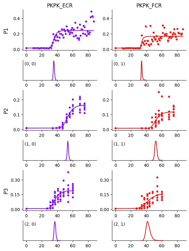
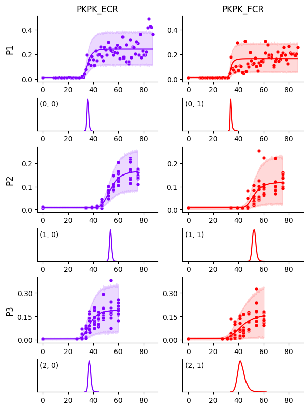
We see that the curve for participant P1 and muscle FCR is no longer biased by those few data points, compared to Getting Started. This becomes even clearer when we plot the HDIs around the curves below.
# Plot observations HDI
output_path = os.path.join(output_dir, "obs_hdi.pdf")
model.plot_curves(
    df=df,
    prediction_df=prediction_df,
    predictive=predictive,
    posterior=posterior,
    encoder=encoder,
    output_path="mixture_obs_hdi.pdf",
    predictive_hdi_var=mep.site.obs,
    predictive_hdi_prob=0.95
)
Accessing parameters#
In this model, the parameter a corresponds to the \(S_{50}\) and can be accessed as below.
# S50 parameter
a = posterior[mep.site.a]
print(a.shape)
(4000, 3, 2)